
I have a data processing problem – I have too much of it. Far far too much… This is a post about exploring data, and how to process a lot of it, using Athena Notebooks which was a fun delve into a world I’d never really tried that much before.
However, to get there, there is a certain amount of setting the scene which is needed. I must ask you to come on a journey of discovery..
The Problem
A project I follow with a certain amount of geeky interest is the WSPRnet which lurks at https://www.wsprnet.org/drupal/wsprnet/map
Essentially the idea is that a small number of very low power radio transmitters send a beacon which other small radio transmitters listen for. The results are collated on a web site and people can download the contact list.
The problem is that it has become, well, popular. Very popular. The filesizes in 2009 a year after it started were on the order of about 50MB a month. Come 2024, and we are knocking on the door of 15GB a month.
The other problem is that people are not using the system as it was designed, and it’s very difficult to fix the issue now. So the data we have is polluted… the old Big Data problem of Buggy Data… it needs cleaning up.
If we look at a typical dump of some of these CSV files we can see the structure
1147599800,1525132920,GM1OXB,IO87ir,-20,7.040096,OM1AI,JN88,23,0,1688,315,7,,0
1146484268,1525132920,G3ZIL,IO90hw,-26,7.040135,WA4KFZ,FM18gv,37,0,5864,50,7,,0
1146484266,1525133160,G3ZIL,IO90hw,-20,7.040096,9A5PH,JN73tt,37,0,1500,308,7,,0
The first column is the spotID which is a unique entry into the database, the second is the UNIX timestamp. The third column is the callsign of the amateur radio station that is receiving and they are the ones that report the “spot” and upload it to the database. The seventh field is the callsign of the transmitting station.
All good. Apart from the slight issue that sometimes, people don’t actually put in the transmitting station and instead insert a message…
1146256824,1525133520,SWL-FN13WE,FN13we,-19,7.040008,AJ8S,EM89bt,27,0,746,57,7,2.0_r1714,0Here, we have a station that does nothing but receive – the SWL means that are a shortwave listening station. They have reported the transmitting station, AJ8S correctly though. Worse however, are stations that place incorrect details into the receiving callsign field such as a location
4401042,1237617240,LITCHFIELD,PH57,-22,10.140174,7L1RLL,PM95so,30,0,5427,191,10,1.1_r1042One solution is to clean the data by weeding out the incorrect transmit and receive callsigns. If we assume that any station that transmits also recevies, we can list all the receive station callsigns and then use that to pick only those stations that are also transmitting stations. In other words, we assume that all stations will be both transmitters and receivers and filter out the nonsensical stuff on either side.
This is easy to do with SQL – it’s bread and butter for a database. We simply load all the CSV files into a table, select a distinct list of recive stations and then use that to select those stations that are also transmitting…
LOAD DATA INFILE '/var/lib/load/wsprspots-2024-12.csv' INTO TABLE spots2

insert into prefix select distinct(rx) from spots2;

insert into spots select spots2.* from spots2 inner join prefix on spots2.tx=prefix.pfx;
We load the datafile into spots2, the SELECT DISTINCT makes sure we have a list of all the receiving stations, with only one in the list, and then we use that to select the final list into SPOTS using the standard inner join.
The only problem? It takes…. forever…..
It is fast, assuming you have enough memory. However, as the size of the monthly files increases, the speed falls dramatically. My database server at home has 128GB of ram, 32 CPU’s and a lot of fast disk – it is entirely memory bound. As soon as the work set gets too large for the memory it slows down considerably.
2009-01 started 03:54:06
2009-02 started 03:56:34
2009-03 started 03:59:11
2009-04 started 04:03:03
2009-05 started 04:07:42

.

.

2024-07 started  12:33:38
2024-08 started  13:54:58
2024-09 started  15:09:49
2024-10 started  16:37:41
2024-11 started  18:25:49
2024-12 started  20:14:00
It takes minutes for the first months from 2009 to run, and many hours for the latter ones. Clearly, a better way would be preferable.
Panda bears…
Modern data processing and analytics runs on Python, using a framework called Pandas. If you ever used the language R, this is easy enough to understand and isn’t much more difficult if you never have used R.
On my laptop, the Python looks like this….
>>> import pandas as pd
>>> import pyarrow
>>> dfRaw = pd.read_csv('d:/python/wsprspots-2009-01.csv', header=None)
Here, we import the necessary libraries, Panda and Pyarrow and then create a dataframe called dfRaw to hold the raw data. This is loaded in from disk. If you are using Windows, don’t put backslashs into the path or it gets messy. Python will happily take “normal” *nix forward slashes in the path and not get confused. Loading the dataframe into memory takes a couple of seconds.
We can examine the size with the shape property and see it is about half a million records and 14 columns
>>> dfRaw.shape
(583455, 14)
Now, we pick a list of unique rx callsigns. Pandas has a convenient method to do this..
>>> dfUniqueRx = dfRaw[2].unique()It really is that simple. We can look at the list of the callsigns by calling print…
>>> print(dfUniqueRx)
['RA6AS' 'W3HH' 'PA3GYK' 'PD4U' 'VK6DI' 'WA2YUN' 'DF3DT' 'HA5CVZ' 'IV3NWV'
 'K1JT' 'W1BW' 'NJ0U' 'K8CYV' 'VE7TIL' 'W1XP' 'W3CSW' 'W3PM' 'G3GXQ'
 'N2KFC' 'DL9ZU' 'DO9ZU' 'G0KTN' 'G3XVL' 'G4SMX' 'SP3LYZ' 'DL8YCA'
 .
 .
 .
 .
 'IK4PMB' 'DK1SFA' 'DL2GX' 'VK4ZW' 'PA3DRL' 'G8IHT' 'DF4TN' 'IZ1ANZ'
 'DK1MBY' 'DJ0MY' 'IZ8GGE' 'HB9PNI' 'G0API' 'DL2TE' 'IK2XDE' 'IN3ACW'
 'DL8BB' 'DH3SUP' 'DF5KF' 'N3ZM' 'K8NYY' 'IW0HJQ' 'DL1RTN' 'G7AQA']
So we now have the raw data loaded in and another dataframe holding a single column of data which is the unique callsign list. We can now use some of the powerful querying and filtering that Pandas has.
>>> dfCleaned = dfRaw.loc[dfRaw[6].isin(dfUniqueRx)]
A single line, that needs a little unpicking. We are going to load the results into a new dataframe called dfCleaned. We do this by taking our raw data in dfRaw and specify that on column 6 – that is the seventh column (because we start counting from zero in Python) – we want to only pick values that are in the list of unique callsigns.
loc[6] selects the column to look at, and we apply the .isin filter and supply the list of callsigns from dfUniqueRx. It is that simple.
>>> dfCleaned.shape
(552314, 14)
>>>
We can see the end result has shrunk from 583455 to 552314 rows, so we discarded 31,141 rows.
The end results looks like what we would expect, and we can dump this dataframe out to a CSV file.
>>> dfCleaned
             0           1       2       3   4          5       6       7   8   9     10   11  12          13
2       2891883  1230768000  PA3GYK  JO21qq -21  10.140130  EA1FAQ  IN71op  27   0  1357   31  10  1.01_r1023
3       2891887  1230768000    PD4U  JO22xe -11   7.040029  EA1FAQ  IN71op  27   0  1425   31   7  1.01_r1023
4       2891874  1230768000   VK6DI  OF88cd -26  10.140177  JE5FLM  PM74ah  37   1  7590  196  10  1.01_r1023
5       2948965  1230768000  WA2YUN  RK39hh -23  10.140177  JE5FLM  PM74ah  37   2  3616  109  10         NaN
6       2891878  1230768000   DF3DT  JO43cc -23   7.040136   K4MOG  EM73qw   0   0  7233   41   7  1.01_r1023
...         ...         ...     ...     ...  ..        ...     ...     ...  ..  ..   ...  ...  ..         ...
583430  3471305  1233446160   G8IHT  IO94gi -26   1.838154    K1JT  FN20qi  40   0  5459   48   1    1.0_r987
583444  3471325  1233446280   KL7OA  BP51be -28  10.140182  7L1RLL  PM95so  30   0  5580   36  10  1.01_r1023
583445  3471320  1233446280   VK6DI  OF88cd -23  10.140179  7L1RLL  PM95so  30   0  7886  201  10  1.01_r1023
583446  3471327  1233446280  IK4PMB  JN54mm -16  10.140231   I4BBO  JN54ks  30   0    31  155  10  1.01_r1023
583447  3471324  1233446280   IQ4AX  JN54lp -13  10.140206   I4BBO  JN54ks  30   0    15  155  10  1.01_r1023

[552314 rows x 14 columns]
>>>
The entire process takes seconds, and is far faster than the disk based process of a SQL database. When running on my laptop, there was less than a second processing on each stage after hitting Enter…
So… whats the problem?
Memory.
All is good until you run out of memory. At this point, pandas will start throwing exceptions because you have to fit it into memory…. and if it’s bigger than system ram, it wont play ball. Note that the process above, which has a raw data frame and a cleaned one, means you are using memory inefficiently because you are holding the data twice over.
With the 2009 datasets, the half million rows are only a few MB in total. Looking at the later data from late 2024, we have raw datasizes of 16GB. On laptop with 32GB of ram, this won’t fit twice over and the system runs out of space.
01/05/2024 01:34 15,245,775,287 wsprspots-2024-04.csvThe solution, is a distributed computing solution that specialises in rally big data… and fortunately there is one called Apache Spark. The problem, is that Spark needs a lot of work to set up, and to use and it needs a lot of understanding. Spark worklopads will scale across multiple compute nodes and it will distribute the compute requirements beyond what any one node can provide. Sounds ideal….
Spark of life
Amazon Web Services finally enters the discussion – so I hope you all stuck with me. AWS has a service called Athena, and AWS Glue which provide serverless analytics for processing big data. You simply load in your data via an S3 bucket, and then let Athena do the heavy lifting.
Athena has two main ways of processing data. One is via SQL queries, which are available in all regions where you can get Athena as far as I know. The Spark interface however is NOT available in all AWS regions – it is not available in London, eu-west-2 for example just yet, and you will need to use Dublin eu-west-1 to make use of this. Something to consider if data soverienty is a thing for you…
First things first – lets get the data into the bucket. I created a bucket called 131273-rawdata in the AWS console making sure this was in the eu-west-1 region.
Getting data in is easy – just use the aws cli, which is in my opinion a wonderfully underrated interface. It does have a few quirks about wildcards though.. Copying a single file is easy.
D:\python>aws s3 cp wsprspots-2009-01.csv s3://131273-rawdata/wspr
upload: .\wsprspots-2009-01.csv to s3://131273-rawdata/wspr
Multiple files, well the way you would expect has an issue.
D:\python>aws s3 cp wsprspots-2009-??.csv s3://131273-rawdata/wspr

The user-provided path wsprspots-2009-??.csv does not exist.
The correct way is to try to copy all the files with a period marker and then specify exclude and deny rules….
D:\python>aws s3 cp . s3://131273-rawdata/wspr/ --recursive --exclude "*" --include "wsprspots-2009-*.csv" --dryrun
(dryrun) upload: .\wsprspots-2009-01.csv to s3://131273-rawdata/wspr/wsprspots-2009-01.csv
(dryrun) upload: .\wsprspots-2009-02.csv to s3://131273-rawdata/wspr/wsprspots-2009-02.csv
.
.
.
(dryrun) upload: .\wsprspots-2009-11.csv to s3://131273-rawdata/wspr/wsprspots-2009-11.csv
(dryrun) upload: .\wsprspots-2009-12.csv to s3://131273-rawdata/wspr/wsprspots-2009-12.csv
This copies all files from the . folder ie the current folder and recurses through all files. It then excludes everything, so nothing is copied, and then you permit by way of the final include some files to copy. The –dryrun marker is essential to test. For more information on the s3 cp wildcards I would look here.. https://docs.aws.amazon.com/cli/latest/reference/s3/#use-of-exclude-and-include-filters
Once we have the data uploaded, open the AWS console and navigate to Athena
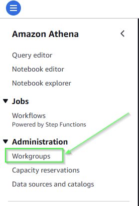
We need to start up an Apache Spark session, which needs a bit of setup work. Click on the hamburger in top left and click on workgroups
Now on the right, click on the yellow Create Workbook and then be sure to select the Apache Spark engine
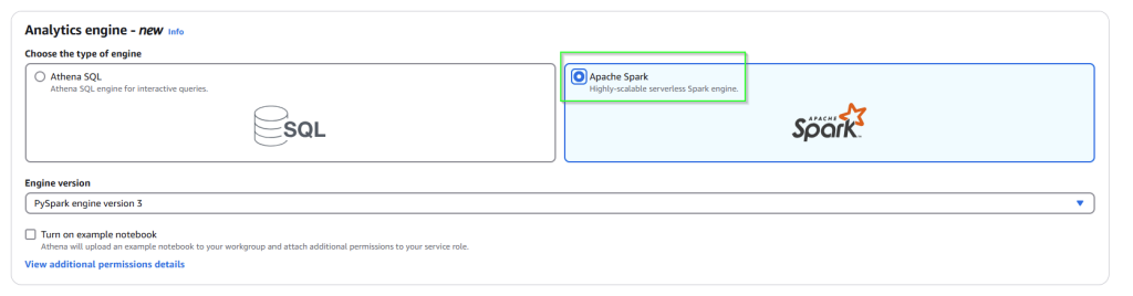
You should then have an Apache Spark enabled workbook.
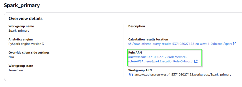
Athena can read files in from a standard S3 bucket, but to put data back into a bucket needs a little more work as it doesnt have the needed permissions. To resolve this open up the workbook page and find the relevant Role ARN
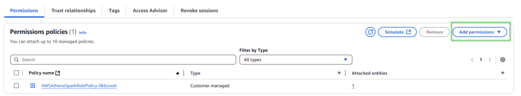
Click on the link and you will end up in the IAM centre
To add the extra permissions in we need to click on the add permission button in Permissions policies.
Specify an Inline policy and then click the JSON tab
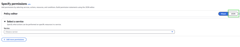
This will show the permissions.
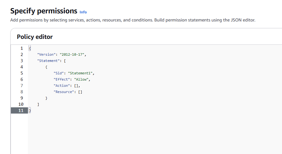
Delete all of the JSON in the Policy Editor, and replace with the following
{
	"Version": "2012-10-17",
	"Statement": [
		{
			"Sid": "VisualEditor0",
			"Effect": "Allow",
			"Action": [
				"s3:GetObject",
				"s3:ListBucket",
				"s3:PutObject",
				"s3:DeleteObject"
			],
			"Resource": [
				"*"
			]
		}
	]
}
This will give a set of reasonably robust permissions that will let Athena write out to any of the S3 buckets you posses – if you want to limit buckets you need to specify specific ones in the Resource section.
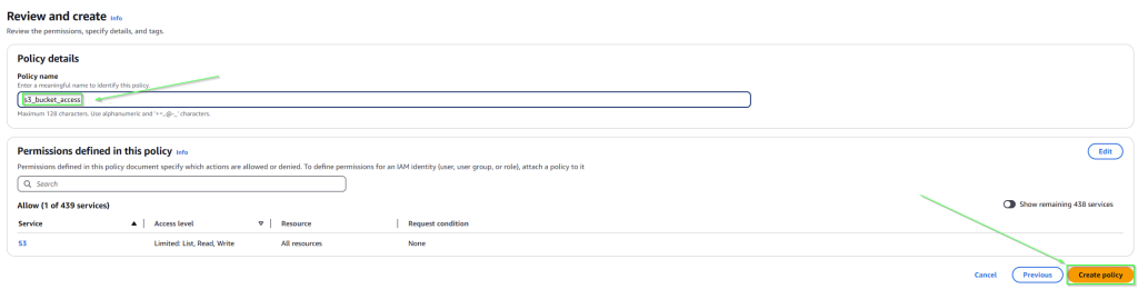
Click on Next and then on the next screen add a name for the policy and then Create Policy
In Athena, navigate on the left to the notebook editor
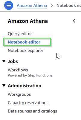
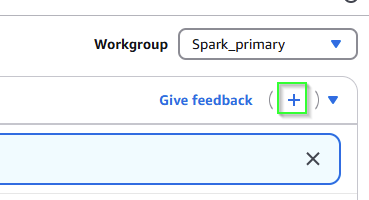
and then on the right, create a new notebook by clicking the plus icon
Once a notebook is created it will have access to up to 20DPUs – these are data processing units that Spark will extend out over if needed to improve the performace. Doing so can be expensive – DPU’s cost per hour and are about $0.55 an hour as well as data scanning of $5 per terabye read. It is possible to limit scale out of DPU’s although a minimum of three must be available.
In the notebook you can add lines which are known as cells. Each cell is sticky – the results stay in there for reuse by subsequent commands.
Here is an example of a notebook in development, the commands are run indivudually to evaluate the output.
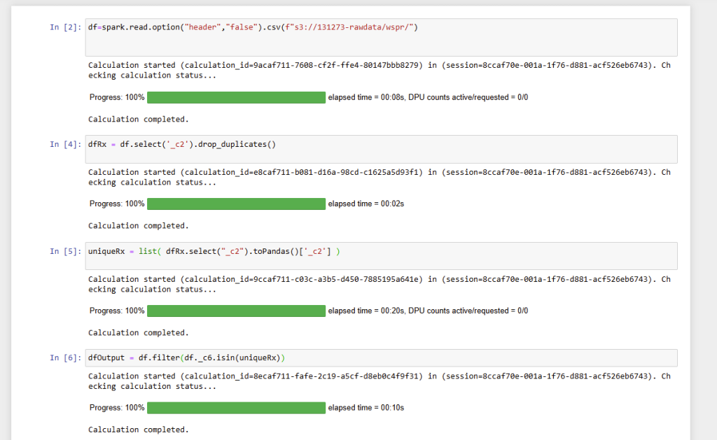
Spark uses a similar structure and way of processing as Pandas, although it is definitly not the same as it has to account for scale out across nodes.
df=spark.read.option("header","false").csv(f"s3://131273-rawdata/wspr/")

dfRx = df.select('_c2').drop_duplicates()

uniqueRx = list( dfRx.select("_c2").toPandas()['_c2'] )

dfOutput = df.filter(df._c6.isin(uniqueRx))

dfOutput.coalesce(1).write.csv(f"s3://131273-rawdata/output.csv")
Line 1 reads in from the S3 bucket. Conveniently if all the files are placed in the same folder, it will read all the CSV files sequentially and process them which is a useful hack
Line 2 selects the duplicates in a similar fashion to the Pandas example earlier
Line3 is a little bit of a hack. You cannot use a Spark dataframe inside another Spark dataframe in Spark, so we convert it to a Pandas frame. This can then be used in line 4 to select the final list.
Finally line 5 writes out the results to the S3 bucket – the coalesce(1) ensures that it writes one file rather than chunking into a series of smaller files.
Apart from the write out – the entire process takes less than 30 seconds to process an entire years data.
Conclusions
Spark for Athena is quick easy and simple to set up and use processing resource. It can easily process data in and out through S3 buckets.
Cost can be an issue – to process a TB of data is going to be $5 to scan it. The the query is run twice then it costs twice as much – this is in addition to the compute costs. It is essential to be sure the queries are going to work without problems.
Local development is therefore essential, which means that you have to have a small Apache Spark setup to develop. This is possible using Python libraries but it is an additional layer of complexity. Small jobs can be prototyped inside of Athena if a small sample dataset is available as data scanning seems to contribute to most of the cost of Athena.
The benefits are large though – you can make use of a hardware setup that would cost upwards of tens of thousands of dollars and make use of it for quite modest outlays. For irregular jobs, it can be quite cost efficient to consume Athena resources for the processing ability that it gives.
Update..
I looked at controlling costs here… https://www.thenetnerd.uk/2025/01/05/parquet-flooring/